Research
RegimeFactorZoo, part two: the replication actually works
A few months ago I wrote a build log for RegimeFactorZoo: the plan, the math, and the WRDS access problem that pushed the whole thing onto public data. That post was written mid-build, on purpose. This one is the receipt.
The foundation is done now, and it holds up. I rebuilt the Fama-French three factors from raw security and accounting data and checked them against Kenneth French's own published series. Then I asked the question that actually matters for a factor: not "does it exist" but "is the risk priced." Then I ran a first small factor zoo on real firm characteristics. Below is what came back, including the number that came out with the wrong sign, which I am leaving in because pretending otherwise would defeat the point of the project.
1. Building the three factors from scratch
The goal of Phase 1 was not to download Ken French's factor returns. Anyone can do that in three lines. The goal was to rebuild them from raw CRSP prices and Compustat fundamentals, so that I actually understood every decision the standard recipe hides.
That means walking the whole thing by hand. Market equity from price times shares, with the CRSP negative-price convention handled (a negative price is a bid-ask midpoint, not a real trade) and the share-count units corrected. Book equity from Compustat using the Davis-Fama-French fallback ladder, keeping only firms with positive book equity. Then book-to-market, timed carefully: book equity from a fiscal year ending in calendar year Y gets paired with market equity from December of that same year, and that pairing is used to sort stocks the following June. The six-month gap is deliberate. It is what stops you from forming a portfolio using a 10-K nobody had filed yet. Finally, NYSE-only breakpoints, a 2×3 sort into six value-weighted portfolios, and out fall SMB and HML.
The part I actually care about is whether it matches. Here is my reconstruction against the published series, cumulative, over 726 overlapping months:
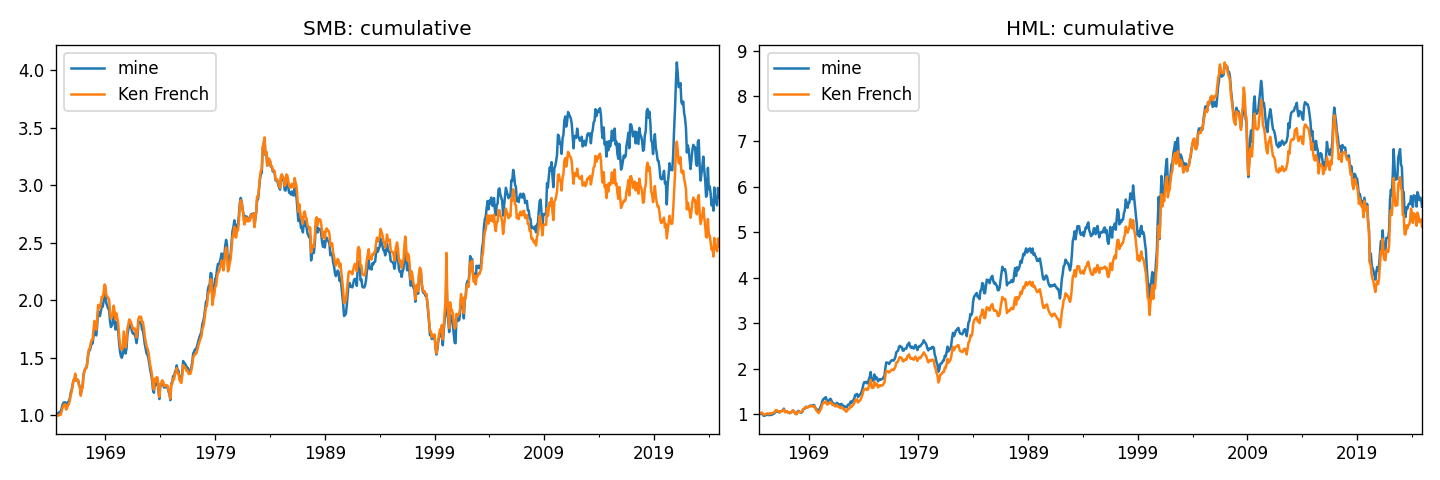
The correlations land at 0.976 for SMB and 0.965 for HML (1964–2024). The few percent of daylight you can see in the SMB panel after 2010 is convention, not error: frozen versus drifting value weights, delisting and micro-cap screens, exactly where breakpoints get drawn. I would be more worried if it matched perfectly.
The sanity checks held all the way down. Apple's December-2023 market cap comes out at $2.98T. Its book-to-market sits near 0.02, which is what you want for an expensive growth stock. And when I sorted on book-to-market, the extreme value names were distressed micro-caps with tiny market caps and stubborn book values, which is exactly who is supposed to be there.
2. Is the risk actually priced?
A factor existing and a factor being rewarded are two different claims. Phase 2 tests the second one with the Fama-MacBeth (1973) two-pass regression.
First pass: for each of the 25 Fama-French size/value test portfolios, regress its excess returns on the three factors over the full history to get its betas. Second pass: for every single month, run a cross-sectional regression of that month's 25 returns on those fixed betas. The slope you get out each month is the price of risk, λ, and stacking them gives a monthly time series. You then average each λ and test it. The one trap here is the standard error: the monthly λ series is autocorrelated, so a naive mean-over-standard-deviation t-stat is too generous. Newey-West standard errors fix that, and they are what I used.
| Factor | Mean λ (monthly) | Newey-West t | Verdict |
|---|---|---|---|
| Market | −0.0062 | −2.07 | Significant, wrong sign |
| SMB (size) | 0.0012 | 0.96 | Not different from zero |
| HML (value) | 0.0033 | 2.20 | Priced |
HML is the clean win: a positive, significant price of risk for value exposure. That is what people mean when they say the value premium is real. SMB comes back indistinguishable from zero in this sample. And the market factor is significant with a negative sign, which is not what any textbook wants.
I want to be honest about that last one rather than bury it. A negative estimated market price of risk is a known and awkward feature of Fama-MacBeth run on these test assets; it says more about the fragility of the estimator on this particular cross-section than about the market not being risky. It is a real result about a real method, so it stays in the table.
3. The factor zoo, one signal at a time
Phase 3 moves down from portfolio-level factors to individual firm characteristics, which is where the "zoo" actually lives. I used the Open Source Asset Pricing panel from Chen and Zimmermann and took nine characteristics. Each one gets lagged a month, so a characteristic measured at month t is used to predict the return at t+1 and never the other way around. Then I winsorized within each month, because a single micro-cap with a 300% monthly return will otherwise hijack the whole cross-section, and ran the same monthly regression per signal with a floor on how many firms a month needs before I trust it.
Eight of the nine come back significant:
| Characteristic | Newey-West t |
|---|---|
| Net debt financing | 8.03 |
| Investment (PPE + inventory) | 7.05 |
| Asset growth | 6.97 |
| Book-to-market | 6.07 |
| Momentum (12-month) | 5.13 |
| Operating profitability | 3.72 |
| Accruals | 2.86 |
| Beta tail risk | 2.79 |
| Cash productivity | 1.40 (not significant) |
Two things I like here. Book-to-market showing up on its own at t = 6.07 closes a loop with Phase 1, where that same signal was doing the work inside HML. And cash productivity failing to clear the bar is, oddly, reassuring. A nine-signal panel where every single characteristic came back significant would be a sign of a leak or a bug, not a triumph. One honest dud is what real data looks like.
(One footgun worth naming: the OSAP file ships its predictors already sign-flipped to point the way theory expects, so asset growth and accruals read positive here instead of with the negative signs you might remember from the original papers. That is the dataset's convention, not a contradiction.)
4. What comes next, now that I've read the paper
The whole project points at Fahiz Baba-Yara, Massimiliano Bondatti, and Robert Hill's In Search of Sparsity, which I have now read cover to cover rather than skimming the abstract. It changed how I think Phases 4 and 5 should go, so let me be precise about what is not built yet.
Phase 4 is the sparse model, and it is not the Lasso regression I had loosely assumed in the first build log. Their method treats the 51 factor-zoo signals as noisy measurements of a small set of latent priced risks, puts a hierarchical spike-and-slab prior on the loading matrix to force most of it to zero, and prices the extracted factors with a Bayesian Fama-MacBeth step. Fifty-one signals collapse to three interpretable latent factors. The right classical warm-up for that is sparse PCA, not Lasso, and that is where I will start.
Phase 5 is the regime question, and reading the paper sharpened it. They already show that the sparse model's implied discount factor is less volatile across the whole sample, so simply re-checking discount-factor volatility in bad markets would just repeat something they have done. The open question is narrower: when you re-estimate the model on different sub-periods, does the loading structure itself move? Do the same signals map to the same latent factors, and do the same factors stay priced? Their sample also ends in 2016, so anything that reaches into the 2020 crash is genuinely new ground.
Both phases are the active build. I am publishing this before they exist because the site is meant to show the work in motion, not a tidy story assembled after the fact.
5. What was actually hard
Most of the pain was in the seams between data sources, which is usually where it is.
Columns coming off CRSP arrive as pandas' nullable Float64 type. Hand one of those to statsmodels or scipy and it quietly casts the whole frame to object and throws. The fix is a one-line defensive .astype("float64") before any regression, and I walked into that wall three separate times before it became muscle memory.
The OSAP book-to-market column had a handful of literal -inf values from a divide-by-almost-zero upstream. Those had to be dropped as missing rather than winsorized, because infinity is not an extreme observation, it is an undefined one, and clipping it would have quietly invented a value.
And the nine-signal panel starts in July 1963 rather than 1926. For a while I assumed I had broken something. I had not: book-to-market needs Compustat coverage, and Compustat coverage begins around 1963. The data was behaving exactly the way real data is supposed to.
References
- Fama, E. F., & French, K. R. (1993). Common Risk Factors in the Returns on Stocks and Bonds. Journal of Financial Economics, 33(1).
- Fama, E. F., & MacBeth, J. D. (1973). Risk, Return, and Equilibrium: Empirical Tests. Journal of Political Economy, 81(3).
- Newey, W. K., & West, K. D. (1987). A Simple, Positive Semi-Definite, Heteroskedasticity and Autocorrelation Consistent Covariance Matrix. Econometrica, 55(3).
- Davis, J. L., Fama, E. F., & French, K. R. (2000). Characteristics, Covariances, and Average Returns: 1929 to 1997. Journal of Finance, 55(1).
- Chen, A. Y., & Zimmermann, T. (2022). Open Source Cross-Sectional Asset Pricing. Critical Finance Review, 11(2).
- Baba-Yara, F., Bondatti, M., & Hill, R. (2026). In Search of Sparsity: Bayesian Sparse Factor Models and the Factor Zoo. Working paper.